NFL2022_stuffs <- read_csv('https://bcdanl.github.io/data/NFL2022_stuffs.csv')Let’s analyze the NFL2022 data:
rmarkdown::paged_table(NFL2022_stuffs) Variable Description for NFL2022_stuffs data.frame
-play_id: Numeric play identifier that when used with game_id and drive provides the unique identifier for a single play
-game_id: Ten digit identifier for NFL game.
-drive: Numeric drive number in the game.
-week: Season week.
-posteam: String abbreviation for the team with possession.
-qtr: Quarter of the game (5 is overtime).
-half_seconds_remaining: Numeric seconds remaining in the half.
-down: The down for the given play. Basically you get four attempts (aka downs) to move the ball 10 yards (by either running with it or passing it). If you make 10 yards then you get another set of four downs.
-pass: Binary indicator if the play was a pass play.
-wp: Estimated winning probability for the posteam given the current situation at the start of the given play.
🏈
Question 2. NFL in 2022
The following is the data.frame for Question 2.
NFL2022_stuffs <- read_csv('https://bcdanl.github.io/data/NFL2022_stuffs.csv')Q2a
In data.frame, NFL2022_stuffs, remove observations for which values of posteam is missing
NFL2022_stuffs <- subset(NFL2022_stuffs, !is.na(posteam))Q2b
Summarize the mean value of pass for each posteam when all the following conditions hold: -wp is greater than 20% and less than 75%; -down is less than or equal to 2; and -half_seconds_remaining is greater than 120.
library(dplyr)

filtered_data <- NFL2022_stuffs %>%
  filter(wp > 0.2 & wp < 0.75, down <= 2, half_seconds_remaining > 120)

summary_data <- filtered_data %>%
  group_by(posteam) %>%
  summarize(mean_pass = mean(pass, na.rm = TRUE))
Q2c
Provide both (1) a ggplot code with geom_point() using the resulting data.frame in Q2b and (2) a simple comment to describe the mean value of pass for each posteam. -In the ggplot, reorder the posteam categories based on the mean value of pass in ascending or in descending order.
summary_data <- summary_data %>%
  arrange(mean_pass)

library(ggplot2)

ggplot(summary_data, aes(x = reorder(posteam, mean_pass), y = mean_pass)) +
  geom_point() +
  labs(title = "Mean Value of pass for Each posteam",
       x = "Percentage of pass plays",
       y = "Team with posession") +
  theme_minimal()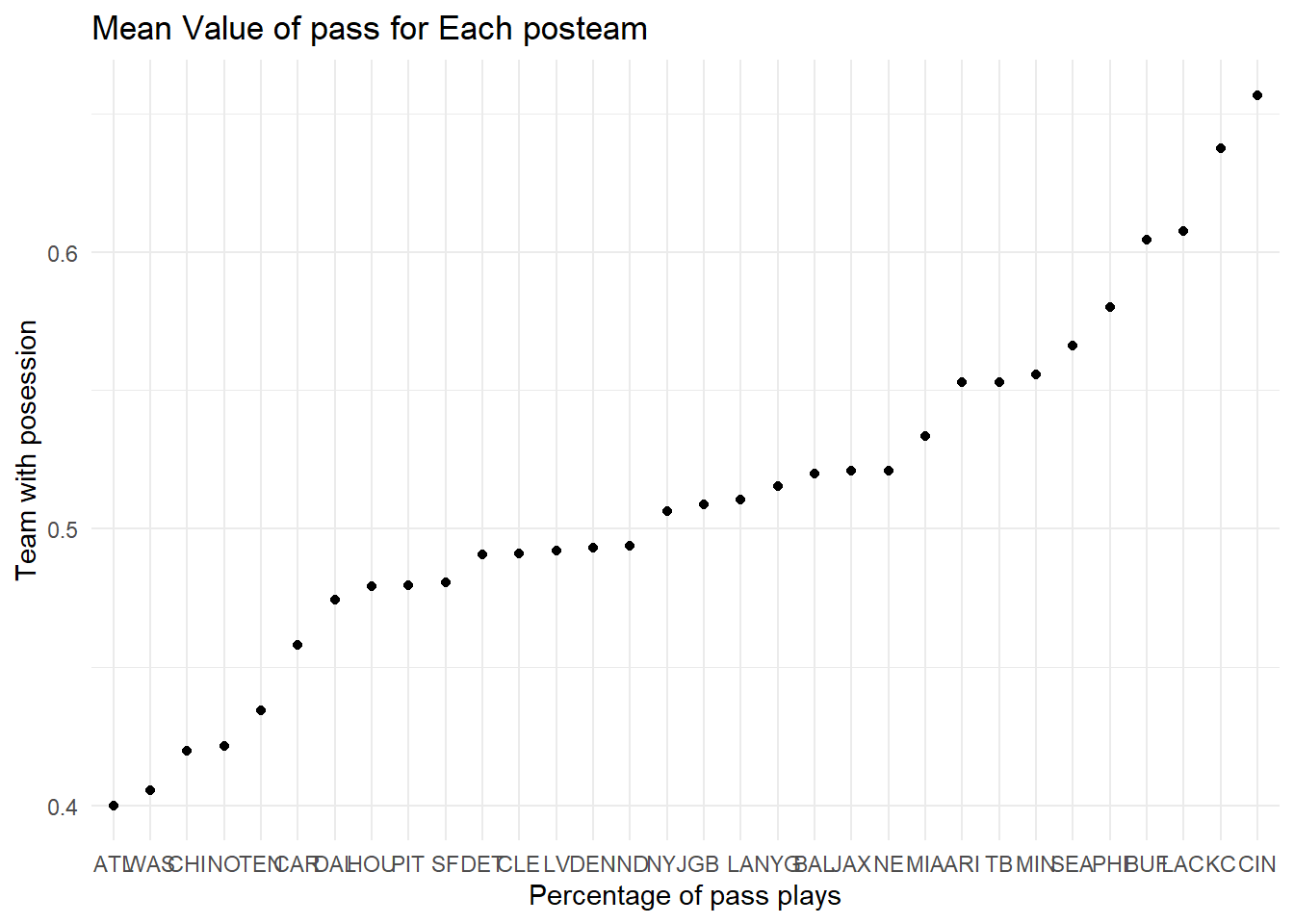
This scatterplot shows that the mean value of pass for each posteam becomes greater, when the team with posession increases their percentage of passing plays.
Q2d
Consider the following data.frame, NFL2022_epa:
NFL2022_epa <- read_csv('https://bcdanl.github.io/data/NFL2022_epa.csv')Create the data.frame, NFL2022_stuffs_EPA, that includes: -All the variables in the data.frame, NFL2022_stuffs; -The variables, passer, receiver, and epa, from the data.frame, NFL2022_epa. by joining the two data.frames. -In the resulting data.frame, NFL2022_stuffs_EPA, remove observations with NA in passer.
library(dplyr)

NFL2022_stuffs_EPA <- merge(NFL2022_stuffs, NFL2022_epa[, c("game_id", "passer", "receiver", "epa")], by = "game_id", all.x = TRUE)
NFL2022_stuffs_EPA <- na.omit(NFL2022_stuffs_EPA)Q2e
Provide both (1) a single ggplot and (2) a simple comment to describe the NFL weekly trend of weekly mean value of epa for each of the following two passers, -“J.Allen” -“P.Mahomes
library(ggplot2)

filtered_data <- NFL2022_stuffs_EPA %>%
  filter(passer %in% c("J.Allen", "P.Mahomes"))

ggplot(filtered_data, aes(x = week, y = epa, color = passer, group = passer)) +
  geom_line() +
  geom_point() +
  labs(title = "Weekly Trend of Mean EPA for J.Allen and P.Mahomes",
       x = "Week",
       y = "Mean EPA") +
  theme_minimal()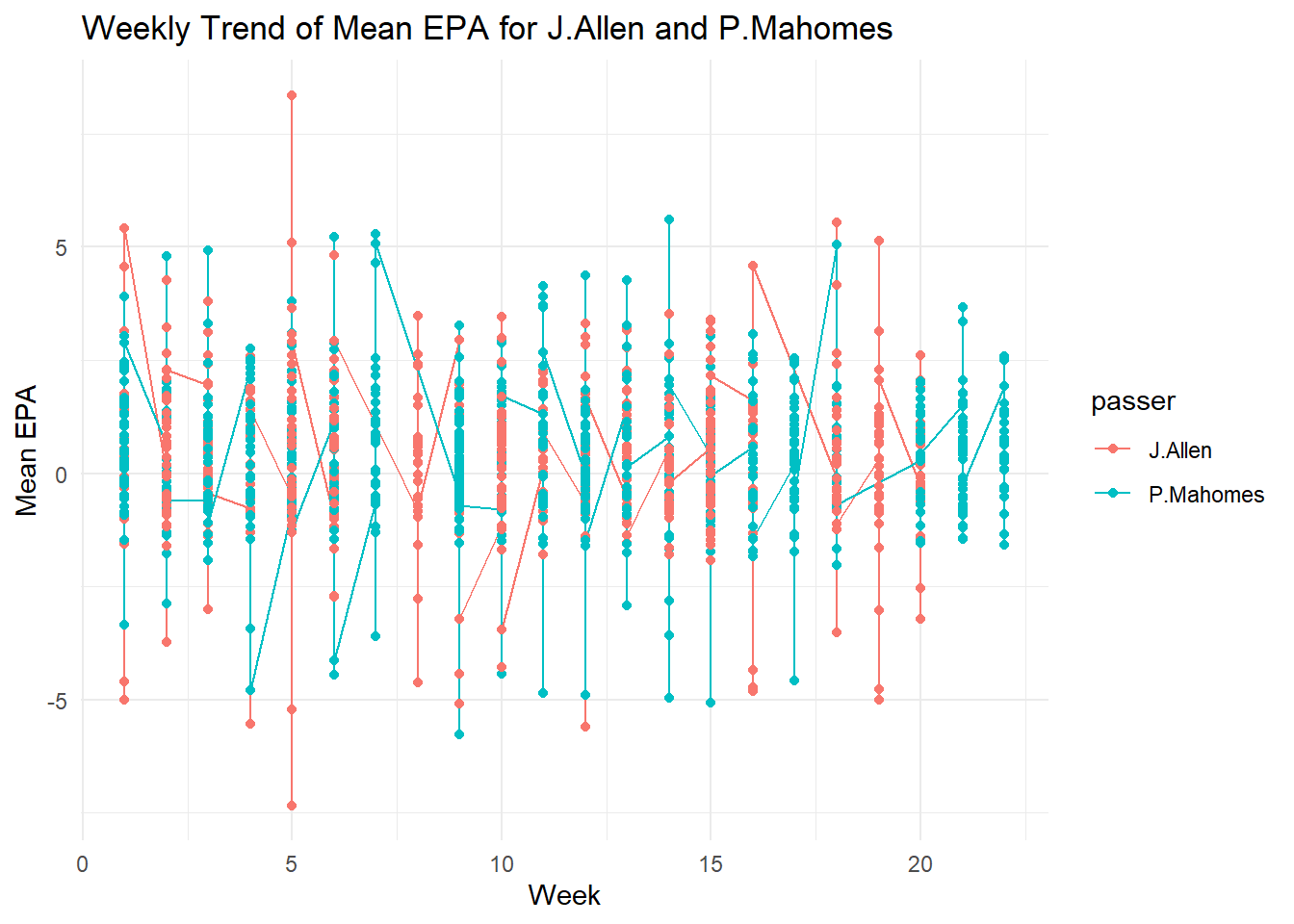
The weekly trend plot illustrates the mean EPA values for passes made by quarterbacks J.Allen and P.Mahomes throughout the NFL 2022 season. We can observe that both quaterbacks follow a similar pattern, with Josh Allen hitting lower lows, and Patrick Mahomes reaching a much higher EPA in the end.
Q2f
Calculate the difference between the mean value of epa for “J.Allen” the mean value of epa for “P.Mahomes” for each value of week.
mean_epa <- filtered_data %>%
  group_by(week, passer) %>%
  summarise(mean_epa = mean(epa, na.rm = TRUE))

mean_epa_wide <- pivot_wider(mean_epa, names_from = passer, values_from = mean_epa)

mean_epa_wide <- mean_epa_wide %>%
  mutate(diff_epa = J.Allen - P.Mahomes)
Q2g
Summarize the resulting data.frame in Q2d, with the following four variables: -posteam: String abbreviation for the team with possession. -passer: Name of the player who passed a ball to a receiver by initially taking a three-step drop, and backpedaling into the pocket to make a pass. (Mostly, they are quarterbacks.) -mean_epa: Mean value of epa in 2022 for each passer -n_pass: Number of observations for each passer
summary_data <- NFL2022_stuffs_EPA %>%
  group_by(posteam, passer) %>%
  summarise(mean_epa = mean(epa, na.rm = TRUE),
            n_pass = n())
Then find the top 10 NFL passers in 2022 in terms of the mean value of epa, conditioning that n_pass must be greater than or equal to the third quantile level of n_pass.
passer_summary <- NFL2022_stuffs_EPA %>%
  group_by(passer) %>%
  summarise(mean_epa = mean(epa, na.rm = TRUE),
            n_pass = n())

quantile_threshold <- quantile(passer_summary$n_pass, 0.75)

top_passers <- passer_summary %>%
  filter(n_pass >= quantile_threshold) %>%
  arrange(desc(mean_epa)) %>%
  head(10)
```